# Load the raw CIFAR-10 data. cifar10_dir = 'cs231n/datasets/cifar-10-batches-py'
# Cleaning up variables to prevent loading data multiple times (which may cause memory issue) try: del X_train, y_train del X_test, y_test print('Clear previously loaded data.') except: pass
# As a sanity check, we print out the size of the training and test data. print('Training data shape: ', X_train.shape) print('Training labels shape: ', y_train.shape) print('Test data shape: ', X_test.shape) print('Test labels shape: ', y_test.shape)
# Output: # Training data shape: (50000, 32, 32, 3) # Training labels shape: (50000,) # Test data shape: (10000, 32, 32, 3) # Test labels shape: (10000,)
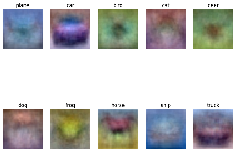
展示一些训练数据样本:
1
2
3
4
5
6
7
8
9
10
11
12
13
14
15
16
# Visualize some examples from the dataset. # We show a few examples of training images from each class. classes = ['plane', 'car', 'bird', 'cat', 'deer', 'dog', 'frog', 'horse', 'ship', 'truck'] num_classes = len(classes) samples_per_class = 7 for y, cls inenumerate(classes): idxs = np.flatnonzero(y_train == y) idxs = np.random.choice(idxs, samples_per_class, replace=False) for i, idx inenumerate(idxs): plt_idx = i * num_classes + y + 1 plt.subplot(samples_per_class, num_classes, plt_idx) plt.imshow(X_train[idx].astype('uint8')) plt.axis('off') if i == 0: plt.title(cls) plt.show()
# Subsample the data for more efficient code execution in this exercise num_training = 5000 mask = list(range(num_training)) X_train = X_train[mask] y_train = y_train[mask]
# Reshape the image data into rows X_train = np.reshape(X_train, (X_train.shape[0], -1)) X_test = np.reshape(X_test, (X_test.shape[0], -1)) print(X_train.shape, X_test.shape)
# Output # (5000, 3072) (500, 3072)
导入kNN分类器,并存储训练数据:
1 2 3 4 5 6 7
from cs231n.classifiers import KNearestNeighbor
# Create a kNN classifier instance. # Remember that training a kNN classifier is a noop: # the Classifier simply remembers the data and does no further processing classifier = KNearestNeighbor() classifier.train(X_train, y_train)
测试阶段
计算每张测试图片与每张训练图片的距离:
1 2 3 4 5 6 7 8 9
# Open cs231n/classifiers/k_nearest_neighbor.py and implement # compute_distances_two_loops.
# Test your implementation: dists = classifier.compute_distances_two_loops(X_test) print(dists.shape)
# In cs231n/classifiers/k_nearest_neighbor.py defcompute_distances_two_loops(self, X): """ Compute the distance between each test point in X and each training point in self.X_train using a nested loop over both the training data and the test data.
Inputs: - X: A numpy array of shape (num_test, D) containing test data.
Returns: - dists: A numpy array of shape (num_test, num_train) where dists[i, j] is the Euclidean distance between the ith test point and the jth training point. """ num_test = X.shape[0] num_train = self.X_train.shape[0] dists = np.zeros((num_test, num_train)) for i inrange(num_test): for j inrange(num_train): ##################################################################### # TODO: # # Compute the l2 distance between the ith test point and the jth # # training point, and store the result in dists[i, j]. You should # # not use a loop over dimension, nor use np.linalg.norm(). # ##################################################################### # L2 distance: d2(I1, I2) = \sqrt{\sum{\square{I^p_1 - I^p_2}}} dists[i, j] = np.sqrt(np.sum(np.square(X[i] - self.X_train[j]))) return dists
回到knn.ipynb,可视化得到的dists:
1 2 3 4
# We can visualize the distance matrix: each row is a single test example and # its distances to training examples plt.imshow(dists, interpolation='none') plt.show()
visualized distance matrix
Inline Question 1
Notice the structured patterns in the distance matrix, where some rows or columns are visibly brighter. (Note that with the default color scheme black indicates low distances while white indicates high distances.)
What in the data is the cause behind the distinctly bright rows?
What causes the columns?
$\color{blue}{\textit Your Answer:}$
Bright rows correspond to test samples that are dissimilar to all training samples. This happens because these test samples may be have high noise, or belong to classes with weak representation in the training set—leading to large distances to all stored training samples.
Bright columns correspond to training samples that are dissimilar to all test samples.
# In cs231n/classifiers/k_nearest_neighbor.py defpredict_labels(self, dists, k=1): """ Given a matrix of distances between test points and training points, predict a label for each test point.
Inputs: - dists: A numpy array of shape (num_test, num_train) where dists[i, j] gives the distance betwen the ith test point and the jth training point.
Returns: - y: A numpy array of shape (num_test,) containing predicted labels for the test data, where y[i] is the predicted label for the test point X[i]. """ num_test = dists.shape[0] y_pred = np.zeros(num_test) for i inrange(num_test): # A list of length k storing the labels of the k nearest neighbors to # the ith test point. closest_y = [] ######################################################################### # TODO: # # Use the distance matrix to find the k nearest neighbors of the ith # # testing point, and use self.y_train to find the labels of these # # neighbors. Store these labels in closest_y. # # Hint: Look up the function numpy.argsort. # ######################################################################### k_nearest_idxs = np.argsort(dists[i])[:k] closest_y = self.y_train[k_nearest_idxs]
######################################################################### # TODO: # # Now that you have found the labels of the k nearest neighbors, you # # need to find the most common label in the list closest_y of labels. # # Store this label in y_pred[i]. Break ties by choosing the smaller # # label. # ######################################################################### counts = np.bincount(closest_y) y_pred[i] = np.argmax(counts)
return y_pred
使用k=1进行预测,查看预测准确率:
1 2 3 4 5 6 7 8 9 10 11
# Now implement the function predict_labels and run the code below: # We use k = 1 (which is Nearest Neighbor). y_test_pred = classifier.predict_labels(dists, k=1)
We can also use other distance metrics such as L1 distance. For pixel values pij(k) at location (i, j) of some image Ik,
the mean μ across all pixels over all images is $$\mu=\frac{1}{nhw}\sum_{k=1}^n\sum_{i=1}^{h}\sum_{j=1}^{w}p_{ij}^{(k)}$$ And the pixel-wise mean μij across all images is $$\mu_{ij}=\frac{1}{n}\sum_{k=1}^np_{ij}^{(k)}.$$ The general standard deviation σ and pixel-wise standard deviation σij is defined similarly.
Which of the following preprocessing steps will not change the performance of a Nearest Neighbor classifier that uses L1 distance? Select all that apply. To clarify, both training and test examples are preprocessed in the same way.
Subtracting the mean μ (p̃ij(k) = pij(k) − μ.)
Subtracting the per pixel mean μij (p̃ij(k) = pij(k) − μij.)
Subtracting the mean μ and dividing by the standard deviation σ.
Subtracting the pixel-wise mean μij and dividing by the pixel-wise standard deviation σij.
Rotating the coordinate axes of the data, which means rotating all the images by the same angle. Empty regions in the image caused by rotation are padded with a same pixel value and no interpolation is performed.
$\color{blue}{\textit Your Answer:}$ 1, 2, 3, 5
$\color{blue}{\textit Your Explanation:}$ The core principle is that preprocessing must preserve the relative magnitudes of L1 distances between samples. Only 4 breaks it.
# In cs231n/classifiers/k_nearest_neighbor.py defcompute_distances_one_loop(self, X): """ Compute the distance between each test point in X and each training point in self.X_train using a single loop over the test data.
Input / Output: Same as compute_distances_two_loops """ num_test = X.shape[0] num_train = self.X_train.shape[0] dists = np.zeros((num_test, num_train)) for i inrange(num_test): ####################################################################### # TODO: # # Compute the l2 distance between the ith test point and all training # # points, and store the result in dists[i, :]. # # Do not use np.linalg.norm(). # ####################################################################### dists[i] = np.sqrt(np.sum(np.square(X[i] - self.X_train), axis=1)) return dists
# Now lets speed up distance matrix computation by using partial vectorization # with one loop. Implement the function compute_distances_one_loop and run the # code below: dists_one = classifier.compute_distances_one_loop(X_test)
# To ensure that our vectorized implementation is correct, we make sure that it # agrees with the naive implementation. There are many ways to decide whether # two matrices are similar; one of the simplest is the Frobenius norm. In case # you haven't seen it before, the Frobenius norm of two matrices is the square # root of the squared sum of differences of all elements; in other words, reshape # the matrices into vectors and compute the Euclidean distance between them. difference = np.linalg.norm(dists - dists_one, ord='fro') print('One loop difference was: %f' % (difference, )) if difference < 0.001: print('Good! The distance matrices are the same') else: print('Uh-oh! The distance matrices are different')
# Output: # One loop difference was: 0.000000 # Good! The distance matrices are the same
# In cs231n/classifiers/k_nearest_neighbor.py defcompute_distances_no_loops(self, X): """ Compute the distance between each test point in X and each training point in self.X_train using no explicit loops.
Input / Output: Same as compute_distances_two_loops """ num_test = X.shape[0] num_train = self.X_train.shape[0] dists = np.zeros((num_test, num_train)) ######################################################################### # TODO: # # Compute the l2 distance between all test points and all training # # points without using any explicit loops, and store the result in # # dists. # # # # You should implement this function using only basic array operations; # # in particular you should not use functions from scipy, # # nor use np.linalg.norm(). # # # # HINT: Try to formulate the l2 distance using matrix multiplication # # and two broadcast sums. # ######################################################################### sum_x2 = np.reshape(np.sum(np.square(X), axis=1), (num_test, 1)) sum_xt2 = np.reshape(np.sum(np.square(self.X_train), axis=1), (1, num_train)) matmul_xxt = np.dot(X, self.X_train.T) dists = np.sqrt(sum_x2 + sum_xt2 - 2 * matmul_xxt) return dists
测试并检查正确性:
1 2 3 4 5 6 7 8 9 10 11 12 13 14 15
# Now implement the fully vectorized version inside compute_distances_no_loops # and run the code dists_two = classifier.compute_distances_no_loops(X_test)
# check that the distance matrix agrees with the one we computed before: difference = np.linalg.norm(dists - dists_two, ord='fro') print('No loop difference was: %f' % (difference, )) if difference < 0.001: print('Good! The distance matrices are the same') else: print('Uh-oh! The distance matrices are different')
# Output: # No loop difference was: 0.000000 # Good! The distance matrices are the same
# Let's compare how fast the implementations are deftime_function(f, *args): """ Call a function f with args and return the time (in seconds) that it took to execute. """ import time tic = time.time() f(*args) toc = time.time() return toc - tic
two_loop_time = time_function(classifier.compute_distances_two_loops, X_test) print('Two loop version took %f seconds' % two_loop_time)
one_loop_time = time_function(classifier.compute_distances_one_loop, X_test) print('One loop version took %f seconds' % one_loop_time)
no_loop_time = time_function(classifier.compute_distances_no_loops, X_test) print('No loop version took %f seconds' % no_loop_time)
# You should see significantly faster performance with the fully vectorized implementation!
# NOTE: depending on what machine you're using, # you might not see a speedup when you go from two loops to one loop, # and might even see a slow-down.
# my Output: # Two loop version took 39.707868 seconds # One loop version took 61.474561 seconds # No loop version took 0.530087 seconds # 说明:运行到one_loop时和Colab连接断开,一会后才继续恢复执行,所以时间有点离谱 # 不过跑前面的的代码块的时候one_loop的时间大概45秒左右(没记错的话)。
X_train_folds = [] y_train_folds = [] ################################################################################ # TODO: # # Split up the training data into folds. After splitting, X_train_folds and # # y_train_folds should each be lists of length num_folds, where # # y_train_folds[i] is the label vector for the points in X_train_folds[i]. # # Hint: Look up the numpy array_split function. # ################################################################################ X_train_folds = np.array_split(X_train, num_folds) y_train_folds = np.array_split(y_train, num_folds)
# A dictionary holding the accuracies for different values of k that we find # when running cross-validation. After running cross-validation, # k_to_accuracies[k] should be a list of length num_folds giving the different # accuracy values that we found when using that value of k. k_to_accuracies = {}
################################################################################ # TODO: # # Perform k-fold cross validation to find the best value of k. For each # # possible value of k, run the k-nearest-neighbor algorithm num_folds times, # # where in each case you use all but one of the folds as training data and the # # last fold as a validation set. Store the accuracies for all fold and all # # values of k in the k_to_accuracies dictionary. # ################################################################################ for k in k_choices: k_to_accuracies[k] = [] for i inrange(num_folds): train_X = np.concatenate([X_train_folds[j] for j inrange(num_folds) if j != i]) train_y = np.concatenate([y_train_folds[j] for j inrange(num_folds) if j != i]) test_X = X_train_folds[i] test_y = y_train_folds[i] classifier = KNearestNeighbor() classifier.train(train_X, train_y) test_y_pred = classifier.predict(X=test_X, k=k, num_loops=0) num_correct = np.sum(test_y_pred == test_y) accuracy = float(num_correct) / len(test_y) k_to_accuracies[k].append(accuracy)
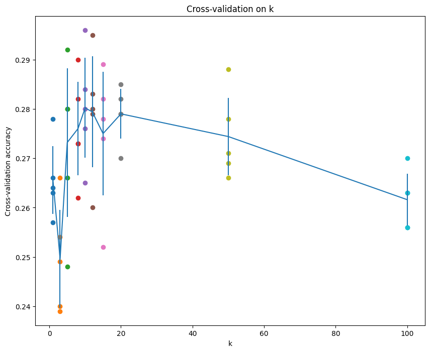
# Print out the computed accuracies for k insorted(k_to_accuracies): for accuracy in k_to_accuracies[k]: print('k = %d, accuracy = %f' % (k, accuracy))
k = 1, accuracy = 0.263000 k = 1, accuracy = 0.257000 k = 1, accuracy = 0.264000 k = 1, accuracy = 0.278000 k = 1, accuracy = 0.266000 k = 3, accuracy = 0.239000 k = 3, accuracy = 0.249000 k = 3, accuracy = 0.240000 k = 3, accuracy = 0.266000 k = 3, accuracy = 0.254000 k = 5, accuracy = 0.248000 k = 5, accuracy = 0.266000 k = 5, accuracy = 0.280000 k = 5, accuracy = 0.292000 k = 5, accuracy = 0.280000 k = 8, accuracy = 0.262000 k = 8, accuracy = 0.282000 k = 8, accuracy = 0.273000 k = 8, accuracy = 0.290000 k = 8, accuracy = 0.273000 k = 10, accuracy = 0.265000 k = 10, accuracy = 0.296000 k = 10, accuracy = 0.276000 k = 10, accuracy = 0.284000 k = 10, accuracy = 0.280000 k = 12, accuracy = 0.260000 k = 12, accuracy = 0.295000 k = 12, accuracy = 0.279000 k = 12, accuracy = 0.283000 k = 12, accuracy = 0.280000 k = 15, accuracy = 0.252000 k = 15, accuracy = 0.289000 k = 15, accuracy = 0.278000 k = 15, accuracy = 0.282000 k = 15, accuracy = 0.274000 k = 20, accuracy = 0.270000 k = 20, accuracy = 0.279000 k = 20, accuracy = 0.279000 k = 20, accuracy = 0.282000 k = 20, accuracy = 0.285000 k = 50, accuracy = 0.271000 k = 50, accuracy = 0.288000 k = 50, accuracy = 0.278000 k = 50, accuracy = 0.269000 k = 50, accuracy = 0.266000 k = 100, accuracy = 0.256000 k = 100, accuracy = 0.270000 k = 100, accuracy = 0.263000 k = 100, accuracy = 0.256000 k = 100, accuracy = 0.263000
可视化一下:
1 2 3 4 5 6 7 8 9 10 11 12 13
# plot the raw observations for k in k_choices: accuracies = k_to_accuracies[k] plt.scatter([k] * len(accuracies), accuracies)
# plot the trend line with error bars that correspond to standard deviation accuracies_mean = np.array([np.mean(v) for k,v insorted(k_to_accuracies.items())]) accuracies_std = np.array([np.std(v) for k,v insorted(k_to_accuracies.items())]) plt.errorbar(k_choices, accuracies_mean, yerr=accuracies_std) plt.title('Cross-validation on k') plt.xlabel('k') plt.ylabel('Cross-validation accuracy') plt.show()
Cross-validation on k
1 2 3 4 5 6 7 8 9 10 11 12 13 14 15 16
# Based on the cross-validation results above, choose the best value for k, # retrain the classifier using all the training data, and test it on the test # data. You should be able to get above 28% accuracy on the test data. best_k = 10
Which of the following statements about k-Nearest Neighbor (k-NN) are true in a classification setting, and for all k? Select all that apply. 1. The decision boundary of the k-NN classifier is linear. 2. The training error of a 1-NN will always be lower than or equal to that of 5-NN. 3. The test error of a 1-NN will always be lower than that of a 5-NN. 4. The time needed to classify a test example with the k-NN classifier grows with the size of the training set. 5. None of the above.
$\color{blue}{\textit Your Answer:}$ 2, 4
$\color{blue}{\textit Your Explanation:}$ When k=1, each prediction is based on solely point, which may lead to overfitting, when increasing k, the classifier gain the ability of generalization, it perform on training may not as good as 1-NN. For k-NN, all computations are in prediction, so once test a example, it needs to calculate distances to all training points.
# Split the data into train, val, and test sets. In addition we will # create a small development set as a subset of the training data; # we can use this for development so our code runs faster. num_training = 49000 num_validation = 1000 num_test = 1000 num_dev = 500
# Our validation set will be num_validation points from the original # training set. mask = range(num_training, num_training + num_validation) X_val = X_train[mask] y_val = y_train[mask]
# Our training set will be the first num_train points from the original # training set. mask = range(num_training) X_train = X_train[mask] y_train = y_train[mask]
# We will also make a development set, which is a small subset of # the training set. mask = np.random.choice(num_training, num_dev, replace=False) X_dev = X_train[mask] y_dev = y_train[mask]
# We use the first num_test points of the original test set as our # test set. mask = range(num_test) X_test = X_test[mask] y_test = y_test[mask]
print('Train data shape: ', X_train.shape) print('Train labels shape: ', y_train.shape) print('Validation data shape: ', X_val.shape) print('Validation labels shape: ', y_val.shape) print('Test data shape: ', X_test.shape) print('Test labels shape: ', y_test.shape)
# Output: # Train data shape: (49000, 32, 32, 3) # Train labels shape: (49000,) # Validation data shape: (1000, 32, 32, 3) # Validation labels shape: (1000,) # Test data shape: (1000, 32, 32, 3) # Test labels shape: (1000,)
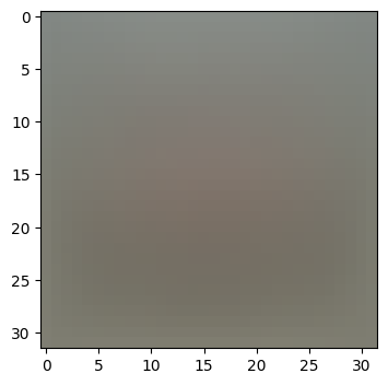
# Preprocessing: subtract the mean image # first: compute the image mean based on the training data mean_image = np.mean(X_train, axis=0) print(mean_image[:10]) # print a few of the elements plt.figure(figsize=(4,4)) plt.imshow(mean_image.reshape((32,32,3)).astype('uint8')) # visualize the mean image plt.show()
# second: subtract the mean image from train and test data X_train -= mean_image X_val -= mean_image X_test -= mean_image X_dev -= mean_image
# third: append the bias dimension of ones (i.e. bias trick) so that our classifier # only has to worry about optimizing a single weight matrix W. X_train = np.hstack([X_train, np.ones((X_train.shape[0], 1))]) X_val = np.hstack([X_val, np.ones((X_val.shape[0], 1))]) X_test = np.hstack([X_test, np.ones((X_test.shape[0], 1))]) X_dev = np.hstack([X_dev, np.ones((X_dev.shape[0], 1))])
# In cs231n/classifiers/softmax.py defsoftmax_loss_naive(W, X, y, reg): """ Softmax loss function, naive implementation (with loops)
Inputs have dimension D, there are C classes, and we operate on minibatches of N examples.
Inputs: - W: A numpy array of shape (D, C) containing weights. - X: A numpy array of shape (N, D) containing a minibatch of data. - y: A numpy array of shape (N,) containing training labels; y[i] = c means that X[i] has label c, where 0 <= c < C. - reg: (float) regularization strength
Returns a tuple of: - loss as single float - gradient with respect to weights W; an array of same shape as W """ # Initialize the loss and gradient to zero. loss = 0.0 dW = np.zeros_like(W)
# compute the loss and the gradient num_classes = W.shape[1] num_train = X.shape[0] for i inrange(num_train): scores = X[i].dot(W)
# compute the probabilities in numerically stable way scores -= np.max(scores) p = np.exp(scores) p /= p.sum() # normalize logp = np.log(p)
loss -= logp[y[i]] # negative log probability is the loss
# compute the gradient for j inrange(num_classes): dW[:, j] += (p[j] - (j == y[i])) * X[i]
# normalized hinge loss plus regularization loss = loss / num_train + reg * np.sum(W * W)
############################################################################# # TODO: # # Compute the gradient of the loss function and store it dW. # # Rather that first computing the loss and then computing the derivative, # # it may be simpler to compute the derivative at the same time that the # # loss is being computed. As a result you may need to modify some of the # # code above to compute the gradient. # ############################################################################# dW = dW / num_train + 2 * reg * W
return loss, dW
测试损失和梯度的计算:
1
2
3
4
5
6
7
8
9
10
11
12
13
14
15
16
17
18
# Evaluate the naive implementation of the loss we provided for you: from cs231n.classifiers.softmax import softmax_loss_naive import time
# generate a random Softmax classifier weight matrix of small numbers W = np.random.randn(3073, 10) * 0.0001
# Once you've implemented the gradient, recompute it with the code below # and gradient check it with the function we provided for you
# Compute the loss and its gradient at W. loss, grad = softmax_loss_naive(W, X_dev, y_dev, 0.0)
# Numerically compute the gradient along several randomly chosen dimensions, and # compare them with your analytically computed gradient. The numbers should match # almost exactly along all dimensions. from cs231n.gradient_check import grad_check_sparse f = lambda w: softmax_loss_naive(w, X_dev, y_dev, 0.0)[0] grad_numerical = grad_check_sparse(f, W, grad)
# do the gradient check once again with regularization turned on # you didn't forget the regularization gradient did you? loss, grad = softmax_loss_naive(W, X_dev, y_dev, 5e1) f = lambda w: softmax_loss_naive(w, X_dev, y_dev, 5e1)[0] grad_numerical = grad_check_sparse(f, W, grad)
Why do we expect our loss to be close to -log(0.1)? Explain briefly.
$\color{blue}{\textit Your Answer:}$When the weights W are initialized to small random values, the logits (scores) computed as X W will be close to zero for all classes. Applying the softmax function to these small logits results in a probability distribution over classes that is approximately uniform. For a 10-class classification task, each class thus has a probability close to 0.1.*
Inline Question 2
Although gradcheck is reliable softmax loss, it is possible that for SVM loss, once in a while, a dimension in the gradcheck will not match exactly. What could such a discrepancy be caused by? Is it a reason for concern? What is a simple example in one dimension where a svm loss gradient check could fail? How would change the margin affect of the frequency of this happening?
Note that SVM loss for a sample (xi, yi) is defined as: Li = ∑j ≠ yimax (0, sj − syi + Δ) where j iterates over all classes except the correct class yi and sj denotes the classifier score for jth class. Δ is a scalar margin. For more information, refer to ‘Multiclass Support Vector Machine loss’ on this page.
Hint: the SVM loss function is not strictly speaking differentiable.
$\color{blue}{\textit Your Answer:}$For SVM loss, in gradcheck, a dimension may fail to match because the numerical precision or the loss function’s not differentiable. This is not an implementation error but an inherent property of the loss function itself. Example, with a single feature, the gradient at a point is discontinuous, leading to potential inconsistencies between the numerical and analytical gradients. Increasing the margin can reduces the probability of kinks occurring, minimizing mismatches.
# In cs231n/classifiers/softmax.py defsoftmax_loss_vectorized(W, X, y, reg): """ Softmax loss function, vectorized version.
Inputs and outputs are the same as softmax_loss_naive. """ # Initialize the loss and gradient to zero. loss = 0.0 dW = np.zeros_like(W)
############################################################################# # TODO: # # Implement a vectorized version of the softmax loss, storing the # # result in loss. # ############################################################################# num_train = X.shape[0] scores = X.dot(W) scores -= np.reshape(np.max(scores, axis=1), (num_train, 1)) p = np.exp(scores) p /= np.reshape(np.sum(p, axis=1), (num_train, 1)) logp = np.log(p) loss -= np.sum(logp[np.arange(num_train), y]) loss = loss / num_train + reg * np.sum(W * W)
############################################################################# # TODO: # # Implement a vectorized version of the gradient for the softmax # # loss, storing the result in dW. # # # # Hint: Instead of computing the gradient from scratch, it may be easier # # to reuse some of the intermediate values that you used to compute the # # loss. # ############################################################################# dscores = p dscores[np.arange(num_train), y] -= 1 dW = X.T.dot(dscores) dW = dW / num_train + 2 * reg * W
# Next implement the function softmax_loss_vectorized; for now only compute the loss; # we will implement the gradient in a moment. tic = time.time() loss_naive, grad_naive = softmax_loss_naive(W, X_dev, y_dev, 0.000005) toc = time.time() print('Naive loss: %e computed in %fs' % (loss_naive, toc - tic))
# Complete the implementation of softmax_loss_vectorized, and compute the gradient # of the loss function in a vectorized way.
# The naive implementation and the vectorized implementation should match, but # the vectorized version should still be much faster. tic = time.time() _, grad_naive = softmax_loss_naive(W, X_dev, y_dev, 0.000005) toc = time.time() print('Naive loss and gradient: computed in %fs' % (toc - tic))
tic = time.time() _, grad_vectorized = softmax_loss_vectorized(W, X_dev, y_dev, 0.000005) toc = time.time() print('Vectorized loss and gradient: computed in %fs' % (toc - tic))
# The loss is a single number, so it is easy to compare the values computed # by the two implementations. The gradient on the other hand is a matrix, so # we use the Frobenius norm to compare them. difference = np.linalg.norm(grad_naive - grad_vectorized, ord='fro') print('difference: %f' % difference)
# Output: # Naive loss and gradient: computed in 0.100571s # Vectorized loss and gradient: computed in 0.019927s # difference: 0.000000
# In cs231n/classifiers/linear_classifier.py deftrain( self, X, y, learning_rate=1e-3, reg=1e-5, num_iters=100, batch_size=200, verbose=False, ): """ Train this linear classifier using stochastic gradient descent.
Inputs: - X: A numpy array of shape (N, D) containing training data; there are N training samples each of dimension D. - y: A numpy array of shape (N,) containing training labels; y[i] = c means that X[i] has label 0 <= c < C for C classes. - learning_rate: (float) learning rate for optimization. - reg: (float) regularization strength. - num_iters: (integer) number of steps to take when optimizing - batch_size: (integer) number of training examples to use at each step. - verbose: (boolean) If true, print progress during optimization.
Outputs: A list containing the value of the loss function at each training iteration. """ num_train, dim = X.shape num_classes = ( np.max(y) + 1 ) # assume y takes values 0...K-1 where K is number of classes ifself.W isNone: # lazily initialize W self.W = 0.001 * np.random.randn(dim, num_classes)
# Run stochastic gradient descent to optimize W loss_history = [] for it inrange(num_iters): X_batch = None y_batch = None
######################################################################### # TODO: # # Sample batch_size elements from the training data and their # # corresponding labels to use in this round of gradient descent. # # Store the data in X_batch and their corresponding labels in # # y_batch; after sampling X_batch should have shape (batch_size, dim) # # and y_batch should have shape (batch_size,) # # # # Hint: Use np.random.choice to generate indices. Sampling with # # replacement is faster than sampling without replacement. # ######################################################################### indices = np.random.choice(num_train, size=batch_size, replace=True) X_batch = X[indices] y_batch = y[indices]
# evaluate loss and gradient loss, grad = self.loss(X_batch, y_batch, reg) loss_history.append(loss)
# perform parameter update ######################################################################### # TODO: # # Update the weights using the gradient and the learning rate. # ######################################################################### self.W -= learning_rate * grad
if verbose and it % 100 == 0: print("iteration %d / %d: loss %f" % (it, num_iters, loss))
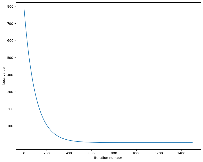
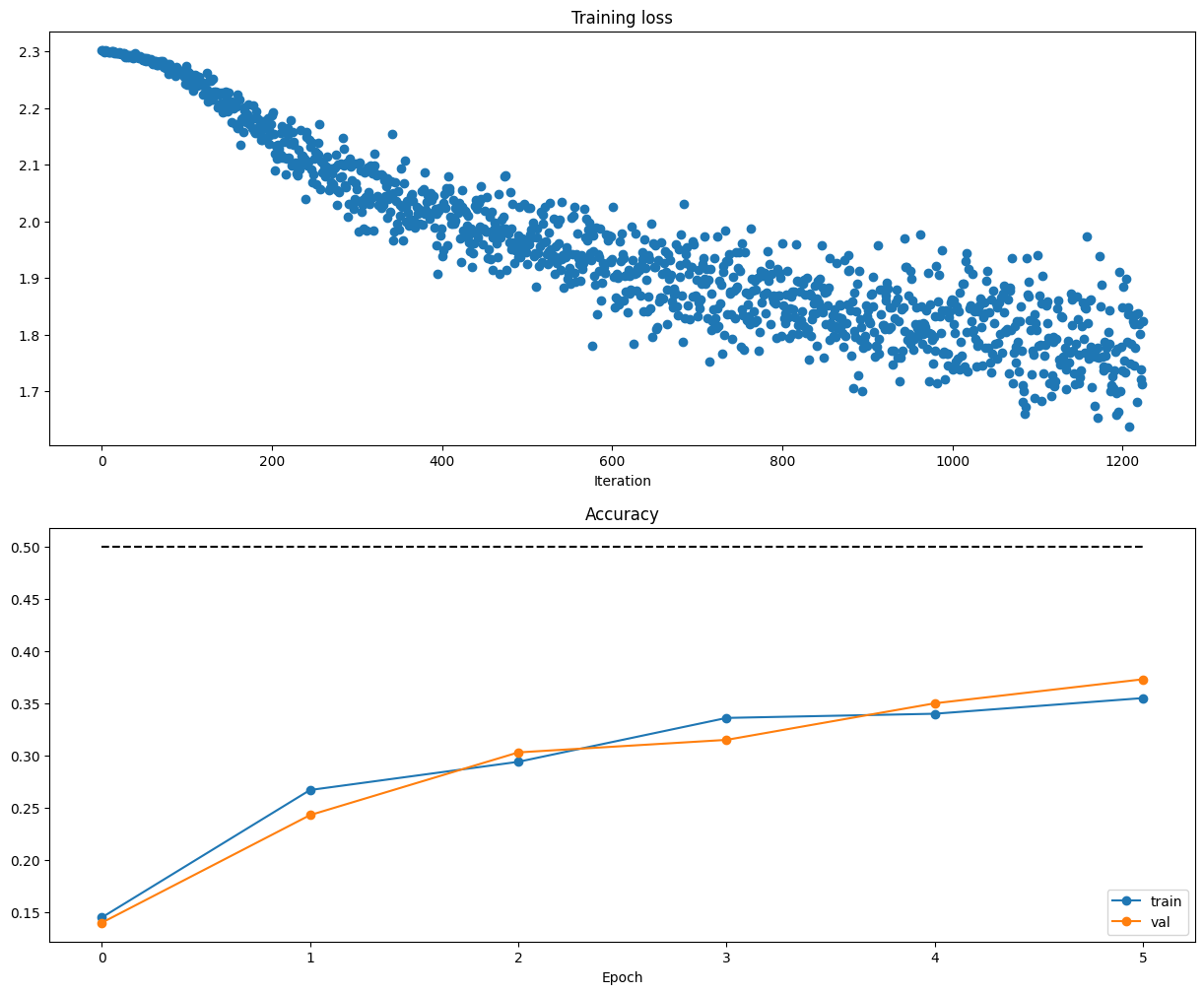
# In the file linear_classifier.py, implement SGD in the function # LinearClassifier.train() and then run it with the code below. from cs231n.classifiers import Softmax softmax = Softmax() tic = time.time() loss_hist = softmax.train(X_train, y_train, learning_rate=1e-7, reg=2.5e4, num_iters=1500, verbose=True) toc = time.time() print('That took %fs' % (toc - tic))
# Output: # iteration 0 / 1500: loss 784.261531 # iteration 100 / 1500: loss 287.556184 # iteration 200 / 1500: loss 106.569326 # iteration 300 / 1500: loss 40.286102 # iteration 400 / 1500: loss 15.996293 # iteration 500 / 1500: loss 7.167806 # iteration 600 / 1500: loss 3.924627 # iteration 700 / 1500: loss 2.739457 # iteration 800 / 1500: loss 2.365508 # iteration 900 / 1500: loss 2.133507 # iteration 1000 / 1500: loss 2.143132 # iteration 1100 / 1500: loss 2.142237 # iteration 1200 / 1500: loss 2.054092 # iteration 1300 / 1500: loss 2.097079 # iteration 1400 / 1500: loss 2.074805 # That took 11.690820s
可视化结果:
1 2 3 4 5 6
# A useful debugging strategy is to plot the loss as a function of # iteration number: plt.plot(loss_hist) plt.xlabel('Iteration number') plt.ylabel('Loss value') plt.show()
# In cs231n/classifiers/linear_classifier.py defpredict(self, X): """ Use the trained weights of this linear classifier to predict labels for data points.
Inputs: - X: A numpy array of shape (N, D) containing training data; there are N training samples each of dimension D.
Returns: - y_pred: Predicted labels for the data in X. y_pred is a 1-dimensional array of length N, and each element is an integer giving the predicted class. """ y_pred = np.zeros(X.shape[0]) ########################################################################### # TODO: # # Implement this method. Store the predicted labels in y_pred. # ########################################################################### scores = X.dot(self.W) y_pred = np.argmax(scores,axis=1)
return y_pred
使用模型预测:
1 2 3 4 5 6 7 8 9 10 11
# Write the LinearClassifier.predict function and evaluate the performance on # both the training and validation set # You should get validation accuracy of about 0.34 (> 0.33). y_train_pred = softmax.predict(X_train) print('training accuracy: %f' % (np.mean(y_train == y_train_pred), )) y_val_pred = softmax.predict(X_val) print('validation accuracy: %f' % (np.mean(y_val == y_val_pred), ))
# Output: # training accuracy: 0.328122 # validation accuracy: 0.343000
# Use the validation set to tune hyperparameters (regularization strength and # learning rate). You should experiment with different ranges for the learning # rates and regularization strengths; if you are careful you should be able to # get a classification accuracy of about 0.365 (> 0.36) on the validation set.
# Note: you may see runtime/overflow warnings during hyper-parameter search. # This may be caused by extreme values, and is not a bug.
# results is dictionary mapping tuples of the form # (learning_rate, regularization_strength) to tuples of the form # (training_accuracy, validation_accuracy). The accuracy is simply the fraction # of data points that are correctly classified. results = {} best_val = -1# The highest validation accuracy that we have seen so far. best_softmax = None# The Softmax object that achieved the highest validation rate.
################################################################################ # TODO: # # Write code that chooses the best hyperparameters by tuning on the validation # # set. For each combination of hyperparameters, train a Softmax on the. # # training set, compute its accuracy on the training and validation sets, and # # store these numbers in the results dictionary. In addition, store the best # # validation accuracy in best_val and the Softmax object that achieves this. # # accuracy in best_softmax. # # # # Hint: You should use a small value for num_iters as you develop your # # validation code so that the classifiers don't take much time to train; once # # you are confident that your validation code works, you should rerun the # # code with a larger value for num_iters. # ################################################################################
# Provided as a reference. You may or may not want to change these hyperparameters learning_rates = [1e-7, 1e-6] regularization_strengths = [2.5e4, 1e4]
for lr in learning_rates: for reg in regularization_strengths: softmax = Softmax() softmax.train(X_train, y_train, learning_rate=lr, reg=reg, num_iters=1500) y_train_pred = softmax.predict(X_train) y_val_pred = softmax.predict(X_val) training_accuracy = np.mean(y_train == y_train_pred) validation_accuracy = np.mean(y_val == y_val_pred) results[(lr, reg)] = (training_accuracy, validation_accuracy) if validation_accuracy > best_val: best_val = validation_accuracy best_softmax = softmax
# Print out results. for lr, reg insorted(results): train_accuracy, val_accuracy = results[(lr, reg)] print('lr %e reg %e train accuracy: %f val accuracy: %f' % ( lr, reg, train_accuracy, val_accuracy))
print('best validation accuracy achieved during cross-validation: %f' % best_val)
# Output: # lr 1.000000e-07 reg 1.000000e+04 train accuracy: 0.356714 val accuracy: 0.371000 # lr 1.000000e-07 reg 2.500000e+04 train accuracy: 0.326122 val accuracy: 0.342000 # lr 1.000000e-06 reg 1.000000e+04 train accuracy: 0.350102 val accuracy: 0.355000 # lr 1.000000e-06 reg 2.500000e+04 train accuracy: 0.321857 val accuracy: 0.334000 # best validation accuracy achieved during cross-validation: 0.371000
# Visualize the cross-validation results import math import pdb
# pdb.set_trace()
x_scatter = [math.log10(x[0]) for x in results] y_scatter = [math.log10(x[1]) for x in results]
# plot training accuracy marker_size = 100 colors = [results[x][0] for x in results] plt.subplot(2, 1, 1) plt.tight_layout(pad=3) plt.scatter(x_scatter, y_scatter, marker_size, c=colors, cmap=plt.cm.coolwarm) plt.colorbar() plt.xlabel('log learning rate') plt.ylabel('log regularization strength') plt.title('CIFAR-10 training accuracy')
# plot validation accuracy colors = [results[x][1] for x in results] # default size of markers is 20 plt.subplot(2, 1, 2) plt.scatter(x_scatter, y_scatter, marker_size, c=colors, cmap=plt.cm.coolwarm) plt.colorbar() plt.xlabel('log learning rate') plt.ylabel('log regularization strength') plt.title('CIFAR-10 validation accuracy') plt.show()
使用得到的表现最好的模型进行测试:
1 2 3 4 5 6 7
# Evaluate the best softmax on test set y_test_pred = best_softmax.predict(X_test) test_accuracy = np.mean(y_test == y_test_pred) print('Softmax classifier on raw pixels final test set accuracy: %f' % test_accuracy)
# Output: # Softmax classifier on raw pixels final test set accuracy: 0.359000
保存模型:
1 2
# Save best softmax model best_softmax.save("best_softmax.npy")
可视化模型学习到的各个类别的权重:
1 2 3 4 5 6 7 8 9 10 11 12 13 14 15
# Visualize the learned weights for each class. # Depending on your choice of learning rate and regularization strength, these may # or may not be nice to look at. w = best_softmax.W[:-1,:] # strip out the bias w = w.reshape(32, 32, 3, 10) w_min, w_max = np.min(w), np.max(w) classes = ['plane', 'car', 'bird', 'cat', 'deer', 'dog', 'frog', 'horse', 'ship', 'truck'] for i inrange(10): plt.subplot(2, 5, i + 1)
# Rescale the weights to be between 0 and 255 wimg = 255.0 * (w[:, :, :, i].squeeze() - w_min) / (w_max - w_min) plt.imshow(wimg.astype('uint8')) plt.axis('off') plt.title(classes[i])
Visualize the learned weights for each class
Inline question 3
Describe what your visualized Softmax classifier weights look like, and offer a brief explanation for why they look the way they do.
$\color{blue}{\textit Your Answer:}$The visualized Softmax classifier weights typically show blurred, low-contrast “templates” that roughly correspond to the key visual features of each class. For example, the weights of class car look like a body of car and its windows. Because the Softmax classifier learns linear decision boundaries. The weights act as feature detectors: during training, each class’s weights adjust to amplify pixel values that are statistically characteristic of that class and suppress irrelevant ones. The blurriness results from the model averaging over diverse training examples, capturing commonalities rather than sharp details. Regularization also smooths the weights, preventing overfitting to noise in the data.
Inline Question 4 - True or False
Suppose the overall training loss is defined as the sum of the per-datapoint loss over all training examples. It is possible to add a new datapoint to a training set that would change the softmax loss, but leave the SVM loss unchanged.
$\color{blue}{\textit Your Answer:}$ True
$\color{blue}{\textit Your Explanation:}$ For the SVM loss, a new datapoint leaves the loss unchanged if, for its true class yi, all other classes j ≠ yi satisfy sj − syi + Δ ≤ 0 (i.e., no margins are violated). In this case, the max(0, ·) term for all j ≠ yi is 0, so the per-datapoint SVM loss is 0, and adding it does not change the total loss. For the softmax loss, however, the loss for a datapoint depends on the probability of its true class ( − log(pyi)), which is never exactly 0 (since softmax probabilities are always positive).
# In cs231n/layers.py defaffine_forward(x, w, b): """ Computes the forward pass for an affine (fully-connected) layer.
The input x has shape (N, d_1, ..., d_k) and contains a minibatch of N examples, where each example x[i] has shape (d_1, ..., d_k). We will reshape each input into a vector of dimension D = d_1 * ... * d_k, and then transform it to an output vector of dimension M.
Inputs: - x: A numpy array containing input data, of shape (N, d_1, ..., d_k) - w: A numpy array of weights, of shape (D, M) - b: A numpy array of biases, of shape (M,)
Returns a tuple of: - out: output, of shape (N, M) - cache: (x, w, b) """ out = None ########################################################################### # TODO: Implement the affine forward pass. Store the result in out. You # # will need to reshape the input into rows. # ########################################################################### out = np.reshape(x, (x.shape[0], -1)).dot(w) + b
########################################################################### # END OF YOUR CODE # ########################################################################### cache = (x, w, b) return out, cache
# In cs231n/layers.py defaffine_backward(dout, cache): """ Computes the backward pass for an affine layer.
Inputs: - dout: Upstream derivative, of shape (N, M) - cache: Tuple of: - x: Input data, of shape (N, d_1, ... d_k) - w: Weights, of shape (D, M) - b: Biases, of shape (M,)
Returns a tuple of: - dx: Gradient with respect to x, of shape (N, d1, ..., d_k) - dw: Gradient with respect to w, of shape (D, M) - db: Gradient with respect to b, of shape (M,) """ x, w, b = cache dx, dw, db = None, None, None ########################################################################### # TODO: Implement the affine backward pass. # ########################################################################### x_reshaped = np.reshape(x, (x.shape[0], -1)) dx = np.reshape(dout.dot(w.T), x.shape) dw = x_reshaped.T.dot(dout) db = np.sum(dout, axis=0)
########################################################################### # END OF YOUR CODE # ########################################################################### return dx, dw, db
# In cs231n/layers.py defrelu_forward(x): """ Computes the forward pass for a layer of rectified linear units (ReLUs).
Input: - x: Inputs, of any shape
Returns a tuple of: - out: Output, of the same shape as x - cache: x """ out = None ########################################################################### # TODO: Implement the ReLU forward pass. # ########################################################################### out = np.maximum(0, x)
########################################################################### # END OF YOUR CODE # ########################################################################### cache = x return out, cache
# In cs231n/layers.py defrelu_backward(dout, cache): """ Computes the backward pass for a layer of rectified linear units (ReLUs).
Input: - dout: Upstream derivatives, of any shape - cache: Input x, of same shape as dout
Returns: - dx: Gradient with respect to x """ dx, x = None, cache ########################################################################### # TODO: Implement the ReLU backward pass. # ########################################################################### dx = dout.copy() dx[x < 0] = 0
########################################################################### # END OF YOUR CODE # ########################################################################### return dx
记得运行测试。
Inline Question 1
We’ve only asked you to implement ReLU, but there are a number of different activation functions that one could use in neural networks, each with its pros and cons. In particular, an issue commonly seen with activation functions is getting zero (or close to zero) gradient flow during backpropagation. Which of the following activation functions have this problem? If you consider these functions in the one dimensional case, what types of input would lead to this behaviour? 1. Sigmoid 2. ReLU 3. Leaky ReLU
$\color{blue}{\textit Your Answer:}$1, 2. For Sigmoid if the input is very large or small(x ≫ 0 or x ≪ 0), the gradient is getting 0. For ReLU if the input is less than 0, the gradient is getting 0.
# In cs231n/layer_utils.py defaffine_relu_forward(x, w, b): """ Convenience layer that perorms an affine transform followed by a ReLU
Inputs: - x: Input to the affine layer - w, b: Weights for the affine layer
Returns a tuple of: - out: Output from the ReLU - cache: Object to give to the backward pass """ a, fc_cache = affine_forward(x, w, b) out, relu_cache = relu_forward(a) cache = (fc_cache, relu_cache) return out, cache
defaffine_relu_backward(dout, cache): """ Backward pass for the affine-relu convenience layer """ fc_cache, relu_cache = cache da = relu_backward(dout, relu_cache) dx, dw, db = affine_backward(da, fc_cache) return dx, dw, db
# In cs231n/layers.py defsoftmax_loss(x, y): """ Computes the loss and gradient for softmax classification.
Inputs: - x: Input data, of shape (N, C) where x[i, j] is the score for the jth class for the ith input. - y: Vector of labels, of shape (N,) where y[i] is the label for x[i] and 0 <= y[i] < C
Returns a tuple of: - loss: Scalar giving the loss - dx: Gradient of the loss with respect to x """ loss, dx = None, None
########################################################################### # TODO: Copy over your solution from A1. ########################################################################### num_train = x.shape[0] scores = x - np.reshape(np.max(x, axis=1), (num_train, 1)) p = np.exp(scores) p /= np.reshape(np.sum(p, axis=1), (num_train, 1)) logp = np.log(p) loss = -np.sum(logp[np.arange(num_train), y]) loss = loss / num_train
dx = p dx[np.arange(num_train), y] -= 1 dx /= num_train ########################################################################### # END OF YOUR CODE # ########################################################################### return loss, dx
# In cs231n/classifiers/fc_net.py classTwoLayerNet(object): """ A two-layer fully-connected neural network with ReLU nonlinearity and softmax loss that uses a modular layer design. We assume an input dimension of D, a hidden dimension of H, and perform classification over C classes.
The architecure should be affine - relu - affine - softmax.
Note that this class does not implement gradient descent; instead, it will interact with a separate Solver object that is responsible for running optimization.
The learnable parameters of the model are stored in the dictionary self.params that maps parameter names to numpy arrays. """
def__init__( self, input_dim=3 * 32 * 32, hidden_dim=100, num_classes=10, weight_scale=1e-3, reg=0.0, ): """ Initialize a new network.
Inputs: - input_dim: An integer giving the size of the input - hidden_dim: An integer giving the size of the hidden layer - num_classes: An integer giving the number of classes to classify - weight_scale: Scalar giving the standard deviation for random initialization of the weights. - reg: Scalar giving L2 regularization strength. """ self.params = {} self.reg = reg
############################################################################ # TODO: Initialize the weights and biases of the two-layer net. Weights # # should be initialized from a Gaussian centered at 0.0 with # # standard deviation equal to weight_scale, and biases should be # # initialized to zero. All weights and biases should be stored in the # # dictionary self.params, with first layer weights # # and biases using the keys 'W1' and 'b1' and second layer # # weights and biases using the keys 'W2' and 'b2'. # ############################################################################ self.params['W1'] = weight_scale * np.random.randn(input_dim, hidden_dim) self.params['b1'] = np.zeros(hidden_dim) self.params['W2'] = weight_scale * np.random.randn(hidden_dim, num_classes) self.params['b2'] = np.zeros(num_classes) ############################################################################ # END OF YOUR CODE # ############################################################################
defloss(self, X, y=None): """ Compute loss and gradient for a minibatch of data.
Inputs: - X: Array of input data of shape (N, d_1, ..., d_k) - y: Array of labels, of shape (N,). y[i] gives the label for X[i].
Returns: If y is None, then run a test-time forward pass of the model and return: - scores: Array of shape (N, C) giving classification scores, where scores[i, c] is the classification score for X[i] and class c.
If y is not None, then run a training-time forward and backward pass and return a tuple of: - loss: Scalar value giving the loss - grads: Dictionary with the same keys as self.params, mapping parameter names to gradients of the loss with respect to those parameters. """ scores = None ############################################################################ # TODO: Implement the forward pass for the two-layer net, computing the # # class scores for X and storing them in the scores variable. # ############################################################################ # first layer: affine - relu W1 = self.params['W1'] b1 = self.params['b1'] h, h_cache = affine_relu_forward(X, W1, b1)
# second layer: affine W2 = self.params['W2'] b2 = self.params['b2'] scores, scores_cache = affine_forward(h, W2, b2) ############################################################################ # END OF YOUR CODE # ############################################################################
# If y is None then we are in test mode so just return scores if y isNone: return scores
loss, grads = 0, {} ############################################################################ # TODO: Implement the backward pass for the two-layer net. Store the loss # # in the loss variable and gradients in the grads dictionary. Compute data # # loss using softmax, and make sure that grads[k] holds the gradients for # # self.params[k]. Don't forget to add L2 regularization! # # # # NOTE: To ensure that your implementation matches ours and you pass the # # automated tests, make sure that your L2 regularization includes a factor # # of 0.5 to simplify the expression for the gradient. # ############################################################################ loss, dscores = softmax_loss(scores, y) loss += 0.5 * self.reg * (np.sum(W1 * W1) + np.sum(W2 * W2))
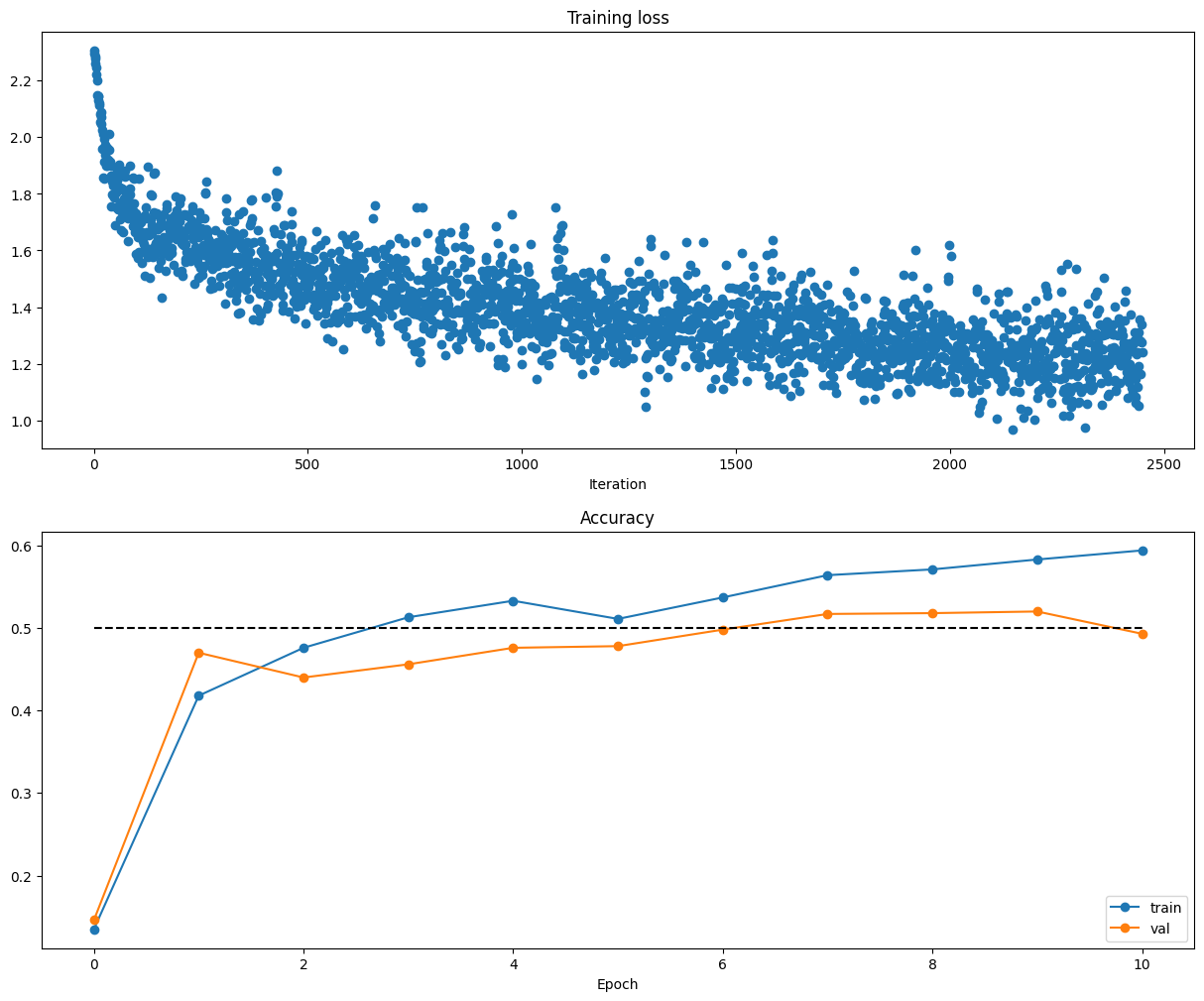
############################################################################## # TODO: Use a Solver instance to train a TwoLayerNet that achieves about 36% # # accuracy on the validation set. # ############################################################################## solver = Solver(model, data, update_rule='sgd', optim_config={ 'learning_rate': 1e-4, }, lr_decay=0.95, num_epochs=5, batch_size=200, print_every=100) solver.train() ############################################################################## # END OF YOUR CODE # ##############################################################################
################################################################################# # TODO: Tune hyperparameters using the validation set. Store your best trained # # model in best_model. # # # # To help debug your network, it may help to use visualizations similar to the # # ones we used above; these visualizations will have significant qualitative # # differences from the ones we saw above for the poorly tuned network. # # # # Tweaking hyperparameters by hand can be fun, but you might find it useful to # # write code to sweep through possible combinations of hyperparameters # # automatically like we did on thexs previous exercises. # ################################################################################# hidden_layer_sizes = [50, 100] learning_rates = [1e-4, 5e-4, 2e-3] training_epochs = [5, 10] regularization_strengths = [5e-3, 1e-2, 2e-2]
for hls in hidden_layer_sizes: for lr in learning_rates: for num_epochs in training_epochs: for reg in regularization_strengths: model = TwoLayerNet(input_size, hidden_dim=hls, num_classes=num_classes, reg=reg) solver = Solver(model, data, update_rule='sgd', optim_config={ 'learning_rate': lr, }, lr_decay=0.95, num_epochs=num_epochs, batch_size=200, print_every=200) solver.train()
# According to the source code of Solver, the final accuracy should be solver.best_val_acc # and the final model parameters will be swapped with the parameters that cause solver.best_val_acc val_accuracy = solver.best_val_acc if val_accuracy > best_val: best_val = val_accuracy best_model = model solver_of_best_model = solver
print('best validation accuracy achieved during cross-validation: %f' % best_val) ################################################################################ # END OF YOUR CODE # ################################################################################
# end of Output: # best validation accuracy achieved during cross-validation: 0.520000
Now that you have trained a Neural Network classifier, you may find that your testing accuracy is much lower than the training accuracy. In what ways can we decrease this gap? Select all that apply.
Train on a larger dataset.
Add more hidden units.
Increase the regularization strength.
None of the above.
$\color{blue}{\textit Your Answer:}$ 1, 3
$\color{blue}{\textit Your Explanation:}$ A larger dataset contains more diverse patterns and reduces the model’s ability to “memorize” noise or idiosyncrasies of the small training set. Regularization constrains the model’s parameter values, preventing it from becoming overly complex and overfitting.
# num_color_bins = 10 # Number of bins in the color histogram num_color_bins = 25# Number of bins in the color histogram feature_fns = [hog_feature, lambda img: color_histogram_hsv(img, nbin=num_color_bins)] X_train_feats = extract_features(X_train, feature_fns, verbose=True) X_val_feats = extract_features(X_val, feature_fns) X_test_feats = extract_features(X_test, feature_fns)
# Preprocessing: Subtract the mean feature mean_feat = np.mean(X_train_feats, axis=0, keepdims=True) X_train_feats -= mean_feat X_val_feats -= mean_feat X_test_feats -= mean_feat
# Preprocessing: Divide by standard deviation. This ensures that each feature # has roughly the same scale. std_feat = np.std(X_train_feats, axis=0, keepdims=True) X_train_feats /= std_feat X_val_feats /= std_feat X_test_feats /= std_feat
test accuracy: 0.418 注:这里测试准确率好像是要求达到0.42及以上,当时眼快了就没继续调了,不过问题不大。
接着保存模型。保存完后可视化一下被错误分类的图片:
1 2 3 4 5 6 7 8 9 10 11 12 13 14 15 16 17 18
# An important way to gain intuition about how an algorithm works is to # visualize the mistakes that it makes. In this visualization, we show examples # of images that are misclassified by our current system. The first column # shows images that our system labeled as "plane" but whose true label is # something other than "plane".
examples_per_class = 8 classes = ['plane', 'car', 'bird', 'cat', 'deer', 'dog', 'frog', 'horse', 'ship', 'truck'] for cls, cls_name inenumerate(classes): idxs = np.where((y_test != cls) & (y_test_pred == cls))[0] idxs = np.random.choice(idxs, examples_per_class, replace=False) for i, idx inenumerate(idxs): plt.subplot(examples_per_class, len(classes), i * len(classes) + cls + 1) plt.imshow(X_test[idx].astype('uint8')) plt.axis('off') if i == 0: plt.title(cls_name) plt.show()
Inline question 1:
Describe the misclassification results that you see. Do they make sense?
$\color{blue}{\textit Your Answer:}$ It makes perfect sense given the visual characteristics of the CIFAR-10 dataset, they are really alike.
然后,训练一个two-layer neural network。
先是预处理一下:
1 2 3 4 5 6 7 8
# Preprocessing: Remove the bias dimension # Make sure to run this cell only ONCE print(X_train_feats.shape) X_train_feats = X_train_feats[:, :-1] X_val_feats = X_val_feats[:, :-1] X_test_feats = X_test_feats[:, :-1]
print(X_train_feats.shape)
接下来基本也是和之前差不多,就是要注意一下调参。
我得到的模型的准确率:
1 2 3
best validation accuracy achieved during cross-validation: 0.605000
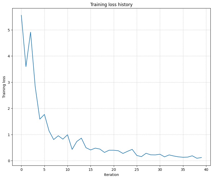
plt.plot(solver.loss_history) plt.title('Training loss history') plt.xlabel('Iteration') plt.ylabel('Training loss') plt.grid(linestyle='--', linewidth=0.5) plt.show()
five-layer network to overfit on a small dataset of 50 images
Inline Question 1: Did you notice anything about the comparative difficulty of training the three-layer network vs. training the five-layer network? In particular, based on your experience, which network seemed more sensitive to the initialization scale? Why do you think that is the case?
Answer: Training the five-layer network is harder. The five-layer network is much more sensitive to initialization scale than the three-layer network. There are some reasons: During backpropagation, gradients get multiplied through more layers, making them prone to explosion (large init) or vanishing (small init); More matrix multiplications allow small errors to accumulate and amplify; Deeper networks have more complex loss landscapes that are highly dependent on initial starting point.
# In cs231n/optim.py defsgd_momentum(w, dw, config=None): """ Performs stochastic gradient descent with momentum.
config format: - learning_rate: Scalar learning rate. - momentum: Scalar between 0 and 1 giving the momentum value. Setting momentum = 0 reduces to sgd. - velocity: A numpy array of the same shape as w and dw used to store a moving average of the gradients. """ if config isNone: config = {} config.setdefault("learning_rate", 1e-2) config.setdefault("momentum", 0.9) v = config.get("velocity", np.zeros_like(w))
next_w = None ########################################################################### # TODO: Implement the momentum update formula. Store the updated value in # # the next_w variable. You should also use and update the velocity v. # ########################################################################### v = config["momentum"] * v - config["learning_rate"] * dw next_w = w + v ########################################################################### # END OF YOUR CODE # ########################################################################### config["velocity"] = v
# In cs231n/optim.py defrmsprop(w, dw, config=None): """ Uses the RMSProp update rule, which uses a moving average of squared gradient values to set adaptive per-parameter learning rates.
config format: - learning_rate: Scalar learning rate. - decay_rate: Scalar between 0 and 1 giving the decay rate for the squared gradient cache. - epsilon: Small scalar used for smoothing to avoid dividing by zero. - cache: Moving average of second moments of gradients. """ if config isNone: config = {} config.setdefault("learning_rate", 1e-2) config.setdefault("decay_rate", 0.99) config.setdefault("epsilon", 1e-8) config.setdefault("cache", np.zeros_like(w))
next_w = None ########################################################################### # TODO: Implement the RMSprop update formula, storing the next value of w # # in the next_w variable. Don't forget to update cache value stored in # # config['cache']. # ########################################################################### cache = config["decay_rate"] * config["cache"] + (1 - config["decay_rate"]) * dw**2 next_w = w - config["learning_rate"] * dw / (np.sqrt(cache) + config["epsilon"])
config["cache"] = cache ########################################################################### # END OF YOUR CODE # ###########################################################################
# In cs231n/optim.py defadam(w, dw, config=None): """ Uses the Adam update rule, which incorporates moving averages of both the gradient and its square and a bias correction term.
config format: - learning_rate: Scalar learning rate. - beta1: Decay rate for moving average of first moment of gradient. - beta2: Decay rate for moving average of second moment of gradient. - epsilon: Small scalar used for smoothing to avoid dividing by zero. - m: Moving average of gradient. - v: Moving average of squared gradient. - t: Iteration number. """ if config isNone: config = {} config.setdefault("learning_rate", 1e-3) config.setdefault("beta1", 0.9) config.setdefault("beta2", 0.999) config.setdefault("epsilon", 1e-8) config.setdefault("m", np.zeros_like(w)) config.setdefault("v", np.zeros_like(w)) config.setdefault("t", 0)
next_w = None ########################################################################### # TODO: Implement the Adam update formula, storing the next value of w in # # the next_w variable. Don't forget to update the m, v, and t variables # # stored in config. # # # # NOTE: In order to match the reference output, please modify t _before_ # # using it in any calculations. # ########################################################################### t = config["t"] + 1 m = config["beta1"] * config["m"] + (1 - config["beta1"]) * dw mt = m / (1 - config["beta1"]**t) v = config["beta2"] * config["v"] + (1 - config["beta2"]) * (dw**2) vt = v / (1 - config["beta2"]**t) next_w = w - config["learning_rate"] * mt / (np.sqrt(vt) + config["epsilon"])
config["m"] = m config["v"] = v config["t"] = t ########################################################################### # END OF YOUR CODE # ###########################################################################
return next_w, config
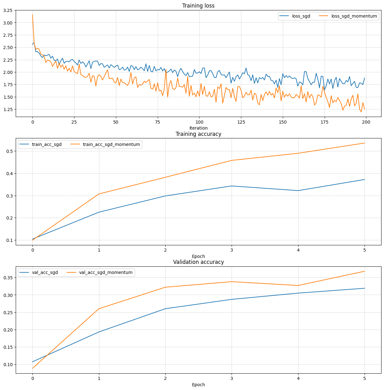
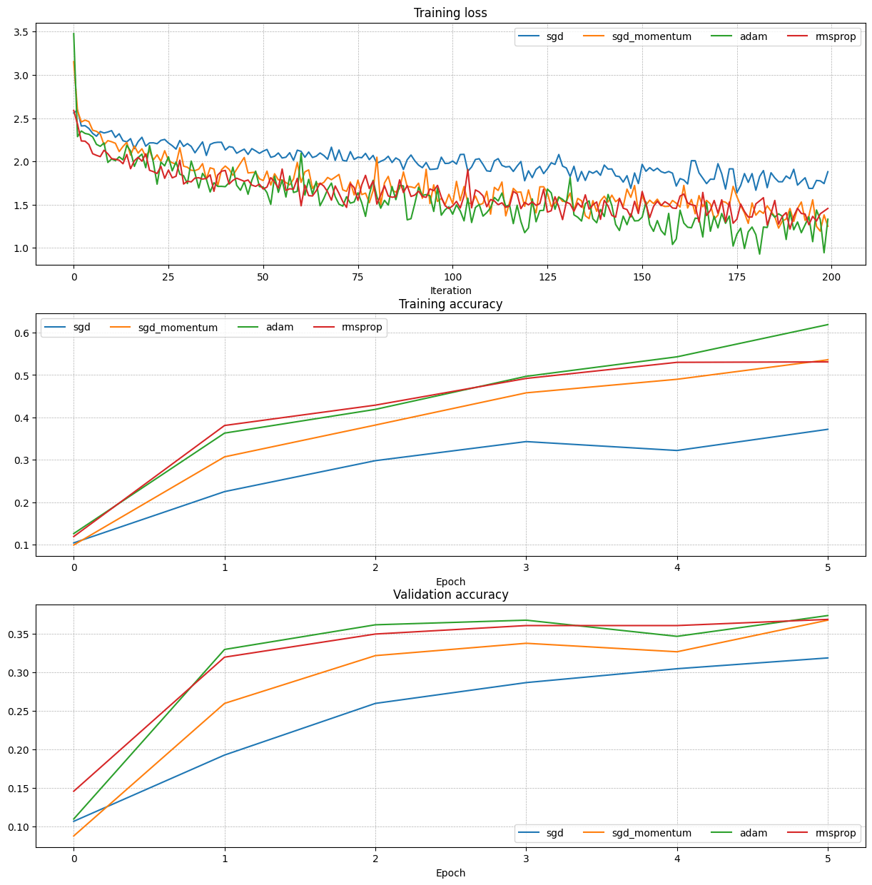
测试正确性后,使用各种优化策略进行对比:
update rules
Inline Question 2:
AdaGrad, like Adam, is a per-parameter optimization method that uses the following update rule:
John notices that when he was training a network with AdaGrad that the updates became very small, and that his network was learning slowly. Using your knowledge of the AdaGrad update rule, why do you think the updates would become very small? Would Adam have the same issue?
Answer: AdaGrad’s updates shrink because cache accumulates squared gradients indefinitely, inflating the denominator. Adam avoids this by using an exponentially weighted average of squared gradients (forgetting old values), keeping updates meaningful.
################################################################################ # TODO: Train the best FullyConnectedNet that you can on CIFAR-10. You might # # find batch/layer normalization and dropout useful. Store your best model in # # the best_model variable. # ################################################################################ # *****START OF YOUR CODE (DO NOT DELETE/MODIFY THIS LINE)***** model = FullyConnectedNet( [512, 256, 100], reg=1e-5, weight_scale=5e-2 ) solver = Solver( model, data, num_epochs=20, batch_size=128, update_rule="adam", optim_config={'learning_rate': 1e-3}, lr_decay=0.95, verbose=True ) solver.train()
best_model = model # *****END OF YOUR CODE (DO NOT DELETE/MODIFY THIS LINE)***** ################################################################################ # END OF YOUR CODE # ################################################################################